Licensed under the Apache License, Version 2.0 (the “License”); you may not use this file except in compliance with the License. You may obtain a copy of the License at http://www.apache.org/licenses/LICENSE-2.0
The reduced transfer function is \[
H(s) = \frac{0.5}{1.010025s^2 + 2.01s + 0.5}
\]
as obtained by:
In [194]:
from sympy import symbols, Matrix, simplify, rootsimport pprints = symbols('s') # Define the Laplace variable 's'# Define the matrix A(s) = s*C + GA_orig = Matrix([ [s +2, 0, -1], [ 0, s +1, -1], [ -1, -1, 0.01* s +2]])A_reduced = Matrix([ [s *1.005+1+0.5, -0.5], [ -0.5, s *1.005+0.5]])def solve(A: Matrix, voltage_row_index: int, current_index: int) ->dict:""" Computes the transfer function H(s) = V_out(s) / J_in(s) for a given system matrix A(s), where V_out(s) is the output voltage and J_in(s) is the input current. Parameters: ---------- A: Matrix The system matrix in the Laplace domain voltage_row_index: int The row index of the inverse matrix A(s)^-1 corresponding to the desired output voltage. For example: - 0 for V_1(s) - 1 for V_2(s) - 2 for V_3(s) current_index: int The column index of the input vector corresponding to the input current. For example: - 0 for J_1(s) - 1 for J_2(s) - 2 for J_3(s) Returns: ------- dict A dictionary containing: - "transfer_function": The symbolic transfer function H(s). - "poles": The poles of the transfer function (roots of the denominator). - "zeros": The zeros of the transfer function (roots of the numerator). - "determinant": The determinant of A(s). - "adjugate": The adjugate matrix of A(s). - "selected_row": The selected row of A(s)^-1 corresponding to the output voltage. - "input_vector": The input vector used in the computation. """ det_A = A.det() # Compute the determinant of A(s) det_A_simplified = simplify(det_A) # Simplify the determinant adj_A = A.adjugate() # Compute the adjugate matrix of A(s) A_inv = adj_A / det_A_simplified # Compute the inverse of A(s) symbolically# Extract the second row of A_inv (e.g., 1 corresponds to V_2(s)) selected_row_A_inv = A_inv.row(voltage_row_index)# Define the input vector [J_1(s), 0, 0] input_vector = Matrix([1if i == current_index else0for i inrange(A.shape[0])])# Compute V_2(s) as the dot product of the second row of A_inv and the input vector V_out_s = simplify(selected_row_A_inv.dot(input_vector)) H_s = V_out_s # Define the transfer function H(s) = V_out(s) / J_in(s) poles = roots(det_A_simplified, s) numerator = simplify(V_out_s.as_numer_denom()[0]) zeros = roots(numerator, s)return {'transfer_function': H_s,'poles': poles,'zeros': zeros,'determinant': det_A_simplified,'adjugate': adj_A,'selected_row': selected_row_A_inv,'input_vector': input_vector }solution_orig = solve(A=A_orig, voltage_row_index=1, current_index=0)solution_redux = solve(A=A_reduced, voltage_row_index=1, current_index=0)pprint.pprint(f"Solution for the original circuit: {solution_orig}\n")pprint.pprint(f"Solution for the reduced circuit: {solution_redux}\n")
import numpy as npimport matplotlib.pyplot as pltfrom scipy.signal import TransferFunction, bode# Generate frequency responsesfreq_range = np.logspace(-2, 3, 500) # Frequency range from 10^-2 to 10^2 rad/sw1, mag1, phase1 = bode( TransferFunction( [1], # H(s) numerator [0.01, 2.03, 4.02, 1.0] # H(s) denominator ), w=freq_range)w2, mag2, phase2 = bode( TransferFunction( [0.5], # H(s) numerator [1.010025, 2.01, 0.5] # H(s) denominator ), w=freq_range)
In [196]:
In [196]:
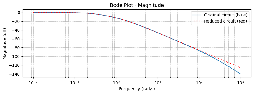
# Plot fT versus Magnitude#| label: fig-bode-plot-ft-vs-mag#| fig-cap: Bode plot: Frequency versus Magnitudeplt.figure(figsize=(10, 3))plt.semilogx(w1, mag1, label='Original circuit (blue)') # Bode magnitude plotplt.semilogx(w2, mag2, color='red', linestyle=':', label='Reduced circuit (red)') # Bode magnitude plotplt.title('Bode Plot - Magnitude')plt.xlabel('Frequency (rad/s)')plt.ylabel('Magnitude (dB)')plt.grid(which='both', linestyle='--', linewidth=0.5)plt.legend()plt.show()
Figure 1
In [197]:
In [197]:
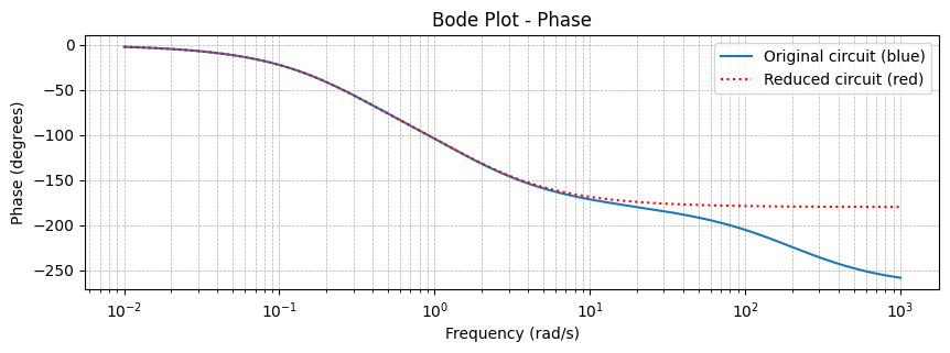
# Plot fT versus phase#| label: fig-bode-plot-ft-vs-phase#| fig-cap: Bode plot: Frequency versus Phaseplt.figure(figsize=(10, 3))plt.semilogx(w1, phase1, label='Original circuit (blue)') # Bode phase plotplt.semilogx(w2, phase2, color='red', linestyle=':', label='Reduced circuit (red)') # Bode phase plotplt.title('Bode Plot - Phase')plt.xlabel('Frequency (rad/s)')plt.ylabel('Phase (degrees)')plt.grid(which='both', linestyle='--', linewidth=0.5)plt.legend()plt.show()
Figure 2
Pole-Zero plots
In [198]:
import matplotlib.pyplot as pltimport numpy as npdef plot_poles_and_zeros(poles, zeros):""" Plots the poles and zeros of a transfer function on the complex plane. Parameters: ---------- poles : list or dict A list or dictionary of poles (roots of the denominator). If it's a dictionary, the keys are the poles, and the values are their multiplicities. zeros : list or dict A list or dictionary of zeros (roots of the numerator). If it's a dictionary, the keys are the zeros, and the values are their multiplicities. Returns: ------- None """# Convert poles and zeros to lists if they are dictionariesifisinstance(poles, dict): poles =list(poles.keys())ifisinstance(zeros, dict): zeros =list(zeros.keys())# Convert symbolic poles and zeros to Python complex numbers poles = [complex(p.evalf()) for p in poles] zeros = [complex(z.evalf()) for z in zeros]# Separate real and imaginary parts for poles and zeros poles_real = [p.real for p in poles] poles_imag = [p.imag for p in poles] zeros_real = [z.real for z in zeros] zeros_imag = [z.imag for z in zeros]# Create the plot plt.figure(figsize=(8, 6)) plt.axhline(0, color='black', linewidth=0.5, linestyle='--') # Horizontal axis plt.axvline(0, color='black', linewidth=0.5, linestyle='--') # Vertical axis# Plot poles and zeros plt.scatter(poles_real, poles_imag, marker='x', color='red', label='Poles', s=100) plt.scatter(zeros_real, zeros_imag, marker='o', color='blue', label='Zeros', s=100)# Add labels and grid plt.title("Pole-Zero Plot") plt.xlabel("Real Part") plt.ylabel("Imaginary Part") plt.grid(True, linestyle='--', alpha=0.7) plt.legend() plt.axis('equal') # Equal scaling for real and imaginary axes# Show the plot plt.show()
In [199]:
In [199]:
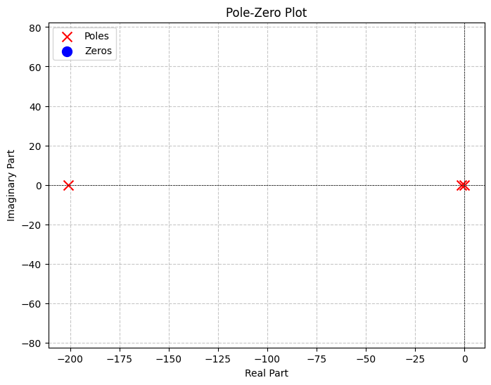
# Pole-Zero Plot for the original circuit#| label: fig-pole-zero-plot-original#| fig-cap: Pole-Zero plot: Original circuitplot_poles_and_zeros(poles=solution_orig['poles'], zeros=solution_orig['zeros'])
Figure 3
If we remove the node at \(s=201\) we get better scaling for comparison.
In [204]:
In [204]:
# Pole-Zero Plot for the original circuit (without the pole at s=201)#| label: fig-pole-zero-plot-original-without-201#| fig-cap: Pole-Zero plot: Original circuit (without the pole at $s = 201$)poles =dict(list(solution_orig['poles'].items())[1:])plot_poles_and_zeros(poles=poles, zeros=solution_orig['zeros'])
Figure 4
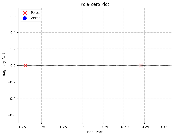
In [200]:
In [200]:
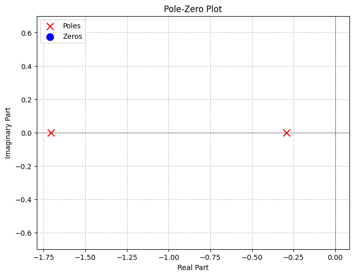
# Pole-Zero Plot for the reduced circuit#| label: fig-pole-zero-plot-reduced#| fig-cap: Pole-Zero plot: Reduced circuitplot_poles_and_zeros(poles=solution_redux['poles'], zeros=solution_redux['zeros'])